Quantum Error Correction
Reliable computations on an unreliable computer\[\newcommand{\B}{\mathbb B} \newcommand{\C}{\mathcal C} \newcommand{\Q}{\mathbb C} \renewcommand{\P}{\mathcal P} \renewcommand{\S}{\mathcal S} \newcommand{\E}{\mathcal E} \newcommand{\X}{\sigma_x} \newcommand{\Z}{\sigma_z} \newcommand{\Y}{\sigma_y} \newcommand{\m}[1]{\begin{bmatrix} #1 \end{bmatrix}} \newcommand{\ket}[1]{\left | #1 \right\rangle} \newcommand{\bra}[1]{\left\langle #1 \right|} \newcommand{\ip}[1]{\left\langle #1 \right\rangle} \newcommand{\op}[2]{\left | #1 \right\rangle \left\langle #2 \right|}\]
Quantum computers promise to solve many problems considered practically impossible using today’s classical computers. However, in constructing such devices, errors are introduced into the system as the unstable subatomic components interact with their environment. Careful encoding of quantum data protects against such errors.
Introduction
Computers have revolutionized society. This much is obvious. They are everywhere from controlling traffic signals to controlling nuclear reactors. They help us compose email and run the stock market. They calculate explosive forces in video games and satellite trajectories. However, there are still many problems just beyond the reach of feasible computation.
One such problem that is difficult on classical computers is simulating quantum systems where the dimensionality of such systems is enormous compared to classical systems. The state of a classical $n$-bit system has dimension $n$ and size $2^n$; however, a quantum $n$-qubit system already has dimension $2^n$ because of complex interactions between quantum states. Simulation of such quantum systems with all these state interactions is largely intractable \cite{Gottesman1997}. If such a system is so hard for us to model on computers, how does Nature seem to do it so easily? This led noted physicist Richard Feynman in 1982 to conjecture that a computer using quantum mechanical processes for computation might be more efficient at such simulations.
A distant possibility in 1982, physical realizations of such quantum computations are now reported every year. However, major hurdles still lay on the path. One of the largest is that of errors creeping into computations: quantum systems are extremely sensitive to their environment. Suppose each computation on a quantum computer introduced some $\epsilon$ of error, then after $N$ computations, the chance of producing an error free result is $(1-\epsilon)^N$ which gets exponentially worse with each further computation.
Digital computers are free from such problems. After each computation, the state is reset to either 0 or 1 and so any small error is corrected. However, a similar problem of error arises in the use of unreliable media. For example, radio transmission in a thunderstorm or reading a scratched compact disc. For these and other such systems, robust encoding schemes have been developed to correct for such errors.
In this report we will briefly cover the development of classical error correcting codes defining several concepts that will lead us to the development of analogous techniques for quantum systems. Included is a survey of several advanced codes and discussion of future directions for fault tolerant quantum computation.
Quantum Channels
Quantum noise, entanglement, and decoherence
Quantum computers are much more sensitive than their classical counterparts, and so errors arise as they interact with their environment while performing computations. While robust advances are announced every year, it is unlikely quantum computers will reach the reliability of classical computers. As such, methods are needed to reliably represent data during storage, computation, and transmission.
The bottom line
Three problems present themselves when designing quantum codes \cite{QCQI}.
- We are unable to replicate an arbitrary state as per the No-Cloning Theorem, hence we cannot simply use replicating an arbitrary qubit to then send. We can however deterministically spread the information contained in some arbitrary state over a larger state space.
- There is a continuum of possible states and hence a continuum of possible errors, and so it is not so simple as detecting which error occurred as some errors could have occurred to greater or lesser extent. Care must be taken in designing a finite set of corrective operations to account for the infinite number of possible errors.
- Directly measurement of qubit states destroys quantum information. While classical coding theory may examine the state of the system and then choose appropriate corrections, quantum coding must be more careful in determining the character of error present. We must measure the error, not the stored information.
Classical Coding Theory
Linear codes
Classical coding theory arose out of the need to communicate data in the presence of noise. Following the pattern of most texts, we consider a unit of data to be a bit, that is, an element of the set $\B=\{0,1\}$, and so all arithmetic is modulo two, i.e. $0+0=1+1=0$ and $0+1=1+0=1$. In this scenario, it is convenient to think of arithmetic as simply bitwise XOR.
A common approach begins by grouping data into uniformly sized blocks of bits. Suppose we wish to encode $k$ bits using $n$ bits where $k<n$. We denote such a scheme as an $[n,k]$ code. In other words, we have a pool of codewords $\C$ of size $2^k$ that we wish to embed in the set $\B^n$ representing $2^n$ possible binary words. If we represent these codewords as binary vectors $v \in \B^k$, it follows naturally to define this encoding as a matrix $G$ called the generator matrix representing the linear transformation $\B^k \rightarrow \B^n$. The original codeword $v$ is now encoded as $Gv \in \B^n$. In effect, this matrix $G$ spreads these codewords out in the higher dimensional space.
Can we now formulate a quick test to see if an arbitrary word $s$ is a codeword? Note that the $k$ columns of $G$ form a basis for the $k$-dimensional subspace of codewords embedded in the $n$-dimensional space of possible words $\B^n$. Let $\C$ denote this embedded codeword subspace. By definition, valid codewords are found strictly within this subspace as a linear combination of these $k$ basis vectors, while invalid codewords will are found at least partly outside this subspace. With this observation, it is interesting to examine this remaining $(n-k)$-dimensional space. Given a generator matrix $G$, we can find the matrix $P$ of maximal rank, the rows of which span this remaining subspace. Then by definition, for codeword $v$, its encoded form $s=Gv$ must be in the null space of $P$, or equivalently $Ps=0$. We now have a quick test to see if arbitrary word $s$ is a valid codeword:
The matrix $P$ is called the parity check matrix.
With this notion of a binary vector space in hand, let’s talk of the nature of errors. Let us define an error $e$ as a contamination of encoded codeword $s \in \C$ to produce $s’ = s + e$. If we perform a parity check on this new word $s’$, we find
\[Ps' = P(s + e) = Ps + Pe = 0 + Pe = Pe .\]The value $Pe$ is called the syndrome of error $e$. Note that if $Pe$ is unique for every possible error $e$, then given arbitrary word $s’$ we can determine and fix whichever error is present. In fact, this is a sufficient condition for error recovery:
Since the value of $Ps’$ depends only on $e$, if $Pe$ is different for all possible errors $e$, then we can uniquely determine which error occurred and fix it.
Another useful way to examine the space of words to look at its topology induced by a norm. Let us now look at such norm, that of Richard Hamming.
Another description of the Hamming distance is the minimum number of bits that must be flipped to convert one word to another. A simpler definition for the minimum Hamming distance is revealed when we remember that since $\C$ is a linear space, $s+t \in \C$ and so $d(s,t)=w(s+t)=w(z)$ for some $z \in \C$. Now the minimum Hamming distance is defined simply as $d(\C)=\min \{ w(s) : s \in \C \}$.
With this notion of distance, we may now quantify the amount of error as the distance between an encoded codeword $s$ and the contaminated version $s’=s+e$. Specifically, the number of errors is
\[d(s',s) = w(s' + s) = w(s + e + s) = w(e) .\]In this sense, errors move a codeword away from its original position. If we assume all errors on to be equally likely, the this perturbation can move the original codeword in any direction. The process of recovering the original codeword is now one of determining the closest codeword. It is often useful to include this minimum distance in the description. Setting $d \equiv d(\C)$ we denote a code now as $[n,k,d]$.
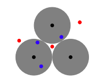
So what does the space of codewords look like? Remember again that the set of valid codewords is spread out in the space of all possible words, any two code words $s,t \in \C$ being a distance of $d(s,t)$ from each other. The figure to the right illustrates a space containing three codewords. In order for us to recover a contaminated codeword, we must be able to trace it back to a unique codeword. This gives rise to the idea that, for a given code, only errors in certain regions are guaranteed to be recoverable. The figure indicates such regions, called Hamming spheres, with shaded circles. For a given code $\C$, all such spheres have radius $r=\tfrac{d(\C)-1}{2}$. In other words, we can correct errors up to size $t$ if $d(\C) \ge 2t+1$. More formally,
Proof: Suppose we have some other codeword in $t \in \C$ that is at least as close to $s'$ as $s$ is, and so may be confused with $s$. In other words $s \ne t$ yet both $d(s,s') = w(e)$ and $d(t,s') \le w(e)$. Then we have $$ 2t < d(\C) \le d(s,t) \le d(s,s') + d(s',t) \le 2w(e) \le 2t $$ implying $2t < 2t$ which is a contradiction. Therefore $s$ is closest to $s'$.
Here our triplet notation $[n,k,d]$ comes in handy. For a code to correct up to $t$ errors, $d > 2t+1$.
One last important concept to define is that of the dual of a code is defined to be the set of all words orthogonal to the code. We denote the dual as $\C^\perp = \{s \in \B^n : s\cdot t=0,\ \forall t \in \C\}$.
We conclude this summary of classical coding theory by mentioning that, in general, the task of finding the original codeword $s$ in an arbitrarily structured space is called the decoding problem and is considered of class NP. Classic coding theory sets out to carefully construct codes with a structure that allows both efficient encoding and decoding. The linear codes described above in terms of generator matrices represent one such class of efficient codes. Along similar lines other methods draw upon abstract algebra using structured groups. And still other approaches use more exotic substrate.
A simple redundant code
The essence of error correction is to encode the data with enough redundancy to ensure recovery in the presence of noise. A straightforward application of this idea is to simply replicate the data. This happens commonly in real life: if you didn’t quite catch what someone just said, you might ask them to repeat it. Let’s now design such a system that encodes a single bit with three copies of itself:
\[\begin{eqnarray*} 0 & \rightarrow & 000 \\ 1 & \rightarrow & 111 . \end{eqnarray*}\]With this setup, we decode the result as the bit with majority presence:
\[\begin{eqnarray*} 000, 100, 010, 001 & \rightarrow & 0 \\ 110, 011, 101, 111 & \rightarrow & 1 . \end{eqnarray*}\]How robust is this system? Suppose we know our noisy channel to flip bits with probability $p > 0$. Majority voting here fails if two or more bits are flipped in error. This system failure occurs with probability $p_f = 3p^2(1-p) + p^3 = 3p^2 - 2p^3$. Compared against the original unprotected version that fails with probability $p$, we want $p_f < p$ which holds if $p < 1/2$.
Quantum Codes
The quantum analogue to linear codes
Here we recast this linear vector space formulation in a manner suitable for addressing quantum systems. In the linear formation, words were considered points in a high dimensional space. In the quantum version, words represent points on the Bloch sphere, i.e. the state of the system. We begin by adopting the bra and ket notation to denote words: $s$ becomes $\ket{s}$. Since bits become qubits, an $n$-bit word $s \in \B^n$ now becomes a $n$-qubit word $\psi \in \Q^{\otimes n}$, the complex Bloch hypersphere. We denote the Pauli operators as $I$, $X=\X$, $Y=\Y$, and $Z=\Z$.
Let us develop a notion of quantum error now. Like any physical quantum process, error is a unitary transformation. Possible such errors may include bit flips, phase flips, or some combination thereof. With the addition of identity $I$ representing no error, these correspond nicely with the Pauli operators: $X$ represents a bit flip, $Z$ represents a phase flip, and $Y$ a combination.
For illustrative purposes, let us begin to design quantum codes for specific errors, the first to address bit flips and the second to address sign changes. Here, as in classic codes, codewords are embedded in a higher dimensional space with special structure.
Three-qubit bit flip code
Let’s design our first quantum code following the pattern of the classic three bit repetition code described in Classic 3bit. In doing so, maybe we can correct for bit flip errors analogous to those of the classical. Remember that we are unable to observe the state of our quantum system directly, so our goal is to reformulate the results from Section \ref{sec:linear_codes} in terms of inner products.
Given arbitrary initial state $\ket{\psi} = a\ket{0} + b\ket{1}$ on the computational basis, where $a,b \in \C$, we first transform it to a new redundant basis $\ket{\psi} = a\ket{000} + b\ket{111}$. This repetition has the effect of spreading the original single qubit state over these three qubits. So as not to destroy the contained information, we must be careful not to perform any direct measurements that would perturb the state. Instead, we carefully measure certain aspects of this augmented state while retaining the original state. Specifically, we measure the difference between certain pairs of qubits.
Recall that errors, like all physical transformations, are unitary operators, hence their action on a system can be undone. Theorem Classical Syndrome tells us that if we can uniquely determine which error syndrome occurred, we can recover the error. Here, as in the classical version, we decode based on which qubit has majority presence, and so here again we assume at most one qubit is in error. In this three qubit encoding, there are the possible errors are: no error, first qubit flipped, second qubit flipped, third qubit flipped. There are four projection operators to detect for these syndromes:
\[\begin{eqnarray*} P_0 \equiv \ket{000}\bra{000} + \ket{111}\bra{111} & \text{no error} \\ P_1 \equiv \ket{100}\bra{100} + \ket{011}\bra{011} & \text{error in first qubit} \\ P_2 \equiv \ket{101}\bra{101} + \ket{101}\bra{101} & \text{error in second qubit} \\ P_3 \equiv \ket{001}\bra{001} + \ket{110}\bra{110} & \text{error in third qubit} \end{eqnarray*}\]Now we must convince ourselves that measuring to test for these error syndromes does not disturb the state of the system. As an example, suppose the first bit was corrupted so that now $\ket{\psi} = a\ket{100} + b\ket{011}$. We then have the following result for syndrome measurement with $P_1$:
\[\begin{align*} \ip{\psi|P_1|\psi} &= \ip{\left(a\bra{100} + b\bra{011}\right) \ket{100}\bra{100} + \ket{011}\bra{011} \left(a\ket{100} + b\ket{011}\right)} \\ &= a^2\ip{100|100} + 2ab\ip{100|011}^2 + b^2\ip{011|011} \\ &= a^2 + b^2 \\ &= 1 . \end{align*}\]Further, $\ip{\psi|P_0|\psi}$, $\ip{\psi|P_2|\psi}$, and $\ip{\psi|P_3|\psi}$ are all zero. Notice that measurement with the syndrome operator $P_1$ does not perturb the state of this corrupted system. This is further confirmed in that the measurement $\ip{\psi|P_1|\psi}$ contains no information as to the $a$ and $b$ of the superimposed state.
Armed with these tests for specific errors, we can design a circuit to apply the appropriate inverse error operation, e.g. $X \otimes I \otimes I$ to un-flip the first qubit.
| Error | $\ip{\psi|Z_{12}|\psi}$ | $\ip{\psi|Z_{12}|\psi}$ |
|---|---|---|
| None | $+1$ | $+1$ |
| First qubit | $-1$ | $+1$ |
| Second qubit | $-1$ | $-1$ |
| Third qubit | $+1$ | $-1$ |
With further work, we can reduce the number of necessary syndrome measurements from four to two. We define two new operators: the first operation compares the first and second qubits, the second operation compares the second and third qubits.
What operators perform this comparison? Remember that the $Z$ operator has spectral decomposition $Z = \op{0}{0} - \op{1}{1}$. Used in a tensor product we get a resulting decomposition that has positive eigenvalues iff the two qubits are the same sign:
\[\begin{align*} Z \otimes Z &= \left( \op{0}{0} - \op{1}{1} \right) \otimes \left( \op{0}{0} - \op{1}{1} \right) \\ &= \op{00}{00} - \op{01}{01} - \op{10}{10} + \op{11}{11} \\ &= \left( \op{00}{00} + \op{11}{11} \right) - \left( \op{01}{01} + \op{10}{10} \right) \end{align*}\]For simplicity of notation involving multi-qubit operators, define an operator $U_i$ to be the tensor product of one qubit operators $U$ acting on qubit $i$ and $I$ acting on the remaining qubits, with analogous extension to multi-qubit operations $U_{ij}$, $U_{ijk}$, etc.. In this notation,
\[Z_{12} = Z \otimes Z \otimes I , \qquad Z_{23} = I \otimes Z \otimes Z ,\]compare the first two qubits and the second two qubits, respectively. Combining the results of these two measurements, we can determine if and where a bit flip occurred. The four possible cases are laid out in the table above. As with the projectors originally defined, measurement with $Z_{12}$ and $Z_{23}$ does not perturb the state. This is an intuitive result as two binary values can form four possible combinations.
Three qubit phase flip code
We now define a quantum code to detect and correct for phase flips, an error that takes $a\ket{0}+b\ket{1}$ to $a\ket{0}-b\ket{1}$. While classical systems do not have a notion of a phase channel, it is interesting that with an appropriate change of basis the phase flip encoding and decoding can simply use the three qubit bit flip code just described. Recall that in the three qubit phase flip code, the error was the $X$ operator performing a bit flip: $\ket{0} \rightarrow \ket{1}$. Notice that if we rotate our computational basis via the Hadamard gate $H$,
\[\begin{eqnarray*} \ket{0} & \rightarrow & \ket{\downarrow} \equiv (\ket{0} + \ket{1})/\sqrt{2} \\ \ket{1} & \rightarrow & \ket{\uparrow} \equiv (\ket{0} - \ket{1})/\sqrt{2} , \end{eqnarray*}\]the phase flip error will analogously be the $HXH$ operation flipping $\ket{\downarrow}$ to $\ket{\uparrow}$ and vice versa. Recall that $H^2=I$, so a second application of the Hadamard operator returns us to the original computational basis. In other words, we can use the three qubit code as a black box by simply rotating before encoding and rotating again after decoding. Where the syndrome measurements were $Z_{ij}$, they are now $H^{\otimes3}~Z_{ij}~H^{\otimes3}$. The transformed syndrome measurements are laid out in the table below. These two codes are said to be unitarily equivalent since the action of one is the same as the other under a unitary change of basis.
| Error | $\ip{\psi|H^{\otimes3}Z_{12}H^{\otimes3}|\psi}$ | $\ip{\psi|H^{\otimes3}Z_{12}H^{\otimes3}|\psi}$ |
|---|---|---|
| None | $+1$ | $+1$ |
| Phase of first qubit | $-1$ | $+1$ |
| Phase of second qubit | $-1$ | $-1$ |
| Phase of third qubit | $+1$ | $-1$ |
The Shor code
Named for its inventor Peter Shor, the Shor code detecting and correcting for both bit flips and phase flips \cite{Shor1995}. In what follows, we outline the technique for a system of one qubit. This scheme is a clever combination of both the bit flip and the phase flip codes described above.
Shor proposed mapping the computational qubit basis into a new basis of two nine-qubit elements. This mapping is broken down into two parts. First we map the computational basis to the phase flip basis,
\[\begin{eqnarray*} \ket{0} & \rightarrow & \ket{\downarrow\downarrow\downarrow} \\ \ket{1} & \rightarrow & \ket{\uparrow\uparrow\uparrow} , \end{eqnarray*}\]then we map each of these qubits to the phase flip code,
\[\begin{eqnarray*} \ket{\downarrow} & \rightarrow & (\ket{000} + \ket{111})/\sqrt{2} \\ \ket{\uparrow} & \rightarrow & (\ket{000} - \ket{111})/\sqrt{2} . \end{eqnarray*}\]The full mapping is then factored as
\[\begin{eqnarray*} \ket{0} & \rightarrow & \frac{(\ket{000} + \ket{111}) (\ket{000} + \ket{111}) (\ket{000} + \ket{111})}{2\sqrt{2}} \\ \ket{1} & \rightarrow & \frac{(\ket{000} - \ket{111}) (\ket{000} - \ket{111}) (\ket{000} - \ket{111})}{2\sqrt{2}} . \end{eqnarray*}\]Before performing some analysis on this representation, let’s first examine a few examples of possible errors and their detection to develop an intuition. Suppose the first qubit is flipped in error, switching $\ket{0…}$ to $\ket{1…}$ and vice versa. For notational While we now have more qubits to test, we still follow the same procedures for checking bit flips and phase flips as in the introductory codes. In this case, we test the sign of the first and second qubits and find $Z_{12}=-1$ indicating one of them flipped. We then check the second two bits and find $Z_{23}=1$ indicating they are of the same sign, and so we conclude that the first bit is flipped and correct it with $X_1$. In the same manner we test for and correct bit flips on the remaining qubits.
As a second example, suppose the first qubit phase was flipped via $Z_1$. Notice that such a phase flip would change the sign of the second element in the first block of three qubits in each factored mapping changing $\ket{000}+\ket{111}$ to $\ket{000}-\ket{111}$ and vice versa. As such, a phase flip in any of the first three qubits would have this affect. Our syndrome test then compares the phase of the first block with the second via $X_{123456}$ and reverses the phase flip via $Z_{123}$. Analogous computations address phase errors in the remaining blocks.
As a final example, suppose the first qubit has both bit flip and phase flip errors, the corrupted state being $Z_1X_1\ket{\psi}$. We show that detection and correction of the bit flip error and the phase flip error may be performed sequentially. Our first syndrome measurement to detect the bit flip error leaves the state untouched, but correcting the bit flip transforms the corrupted state
\[\begin{align*} Z_1X_1\ket{\psi} \rightarrow X_1 Z_1X_1\ket{\psi} &= -Z_1X_1X_1\ket{\psi} \\ &= -Z_1\ket{\psi} , \end{align*}\]since the Pauli operators anti-commute, i.e. $\{X,Z\} = XZ + ZX = 0$. Now notice that our syndrome measurement to detect the phase error on this new state $\ket{\psi’}\equiv -Z_1\ket{\psi}$ is equivalent to detecting the phase error on the original corrupted state:
\[\begin{align*} \ip{\psi'|X_{123456}|\psi'} &= \ip{\psi|Z_1^\dagger X_{123456}Z_1|\psi} \\ &= \ip{\psi|Z_1^\dagger X_1 Z_1 X_{23456}|\psi} \\ &= -\ip{\psi|Z_1^\dagger Z_1 X_1 X_{23456}|\psi} \\ &= -\ip{\psi|Z_1^\dagger X_{23456} Z_1 X_1 |\psi} \\ &= -\ip{\psi|Z_1^\dagger X_1^\dagger X_{123456} Z_1 X_1 |\psi} \\ &= -\ip{\psi|(X_1Z_1)^\dagger X_{123456} (Z_1 X_1) |\psi} \\ &= \ip{\psi|(Z_1X_1)^\dagger X_{123456} (Z_1 X_1) |\psi} . \end{align*}\]Upon detection, the phase is fixed by applying the operator $Z_{123}$.
How robust is this code? Since we compare neighboring qubits to see if their sign is different, the code breaks down if more than one qubit in this 9-qubit tuple is in err. If each qubit decoheres with probability $p$, then the probability that one or zero qubits decohere is $9p(1-p)^8 + (1-p)^9 = (1-p)^8(8p+1)$ and so the probability that two or more qubits decohere leading to erroneous decoding is $1-(1-p)^8(8p+1)~\approx~36p^2$. So, for a $k$-qubit message that we encoded into $9k$-qubits, our chance of successfully decoding the original message is $(1-36p^2)^k$.
Some generalizations
Here we generalize the notion of error and show that the Shor code can correct arbitrary error. Errors, like any action on a quantum system, are unitary operations and as such they can be represented as a linear combination of the Pauli operators operating on the Bloch sphere. Recall that the state of an arbitrary operation has Bloch representation as the density matrix
\[\begin{equation} \rho = \frac{I + \vec{r} \cdot \vec{\sigma}}{2} \end{equation}\]where $\vec{r}$ is a real vector weighting the contribution of each Pauli operator. Now, for an arbitrary error corrupting qubit $i$, we may write
\[\begin{equation} E_i = e_{i0}I + e_{i1}X + e_{i2}Y + e_{i3}Z . \end{equation}\]This leads the transformation that corrupts qubit $i$
\[\begin{equation*} \ket{\psi} = a\ket{0} + b\ket{1} \rightarrow e_{i0}\ket{\psi} + e_{i1}X_i\ket{\psi} + e_{i2}Y_i\ket{\psi} + e_{i3}Z_i\ket{\psi} . \end{equation*}\]With this corrupted state, we begin testing for the presence of the various syndromes on each qubit. For all tests on qubits other than the $i$-th, measurements return zero. Notice that in the previous scenarios, our syndrome measurements leave the state of the system unharmed because each error was either present or not resulting in either 1 or 0 for the measurement. Here, the linear transformation leads to our system collapsing to the measured value with some probability. We measure our system to be
\[\begin{eqnarray*} X_i\ket{\psi} & \text{with probability } |a|^2, \\ Y_i\ket{\psi} & \text{with probability } |b|^2, \\ Z_i\ket{\psi} & \text{with probability } |c|^2, \text{ or } \\ \ket{\psi} & \text{with probability } |d|^2 . \end{eqnarray*}\]The collapsed system is then corrected appropriately \cite{Gottesman1997}.
Example Codes
In this section we document several proposed quantum coding schemes in an effort to illustrate the landscape of such methods. Where appropriate we will document similarities and contrasts between the techniques.
Calderbank-Shor-Steane
Drawing upon classic algebraic coding theory, CSS codes were invented by Calderbank and Shor and simultaneously by Steane. They provide a general formulation for constructing quantum codes from the linear codes readily available \cite{QCQI}. Suppose we have two classic linear codes $\C_1=[n,k_1]$ and $\C_2=[n,k_2]$ where $\C_2 \subset \C_1$ and both $\C_1$ and $\C_2^\perp$ correct for errors of weight $t$, as judged by the Hamming distance. We will now construct an $[n,k_1-k_2]$ quantum code denoted $CSS(\C_1,\C_2)$ capable of correcting $t$ qubit errors.
Recall that in classic codes, each codeword lives in its own subspace. A basis can then be formed for codewords, each codeword then is formed from a linear combination of these basis elements. We can think of these basis elements as cosets with generator words. $\C_2$ then generates cosets for elements $x \in \C_1$:
\[\begin{equation*} \ket{x + \C_2} \equiv \frac{1}{\sqrt{\C_2}} \sum_{y \in \C_2} \ket{x + y} . \end{equation*}\]These cosets are orthonormal. To see this, suppose $x$ and $x’$ are in different cosets of $\C_2$, then by definition, $\nexists y \in \C_2$ such that $x+y=x’+y’$ for any $y’ \in \C_2$. In other words, we can not form linear combinations to equate elements from the two sets, hence they are orthonormal sets.
Now we begin to define the quantum code. Define our new code $CSS(\C_1,\C_2)$ to be spanned by the cosets $\ket{x + \C_2}$. The number of such cosets is $\frac{|\C_1|}{|\C_2|} = \frac{2^{k_1}}{2^{k_2}} = 2^{k_1 - k_2}$, thus our code may be denoted as $[n,k_1-k_2]$.
We now step through examples using this code to correct for both bit flip and phase flip errors, each in turn. Following the classic formulation, an error is a vector that perturbs elements of our codeword. We only need to show that we correct for basis codewords (cosets) since all other codewords are formed as linear combinations. Denote a basis codeword as
\[\begin{equation*} \ket{x+\C_2} = \frac{1}{\sqrt{|\C_2|}} \sum_{y \in \C_2} \ket{x+y} . \end{equation*}\]Suppose this is corrupted by a bit flip error $e_1$. It then becomes,
\[\begin{equation*} \ket{x+\C_2+e_1} = \frac{1}{\sqrt{|\C_2|}} \sum_{y \in \C_2} \ket{x+y+e_1} . \end{equation*}\]If $H_1$ is the parity check matrix for $\C_1$, we can construct a quantum circuit with zero ancilla to perform
\[\begin{eqnarray*} \ket{x+y+e_1}\ket{0} & \rightarrow & \ket{x+y+e_1}\ket{H_1(x+y+e_1)} \\ & & \ket{x+y+e_1}\ket{H_1e_1} , \end{eqnarray*}\]since $x,y \in \C_1$ so $H_1x=H_1y=0$. We measure the ancilla to find $\ket{H_1e_1}$ telling us which error is present and the remaining state is now
\[\begin{equation*} \frac{1}{\sqrt{|\C_2|}} \sum_{y \in \C_2} \ket{x+y+e_1} \end{equation*}\]which can be corrected with appropriate bit flip operations to leave our original state,
\[\begin{equation*} \frac{1}{\sqrt{|\C_2|}} \sum_{y \in \C_2} \ket{x+y} = \ket{x+\C_2} . \end{equation*}\]Suppose now instead that we had a phase flip error. Similar to the Shor’s algorithm \ref{sec:shor}, we rotate our state via Hadamard gates, treat the problem again as a bit flip error, and rotate back after correction.
Before beginning, let’s prove two equalities that will come in handy during the reductions. Recall from our discussion of classical codes that a code $\C$ and its dual $\C^\perp$ are orthogonal spaces. Suppose $y \in \C$ and $z \in \C^\perp$. Then $y\cdot z=0$, and so consequently, $\sum_{y \in \C}(-1)^{z\cdot y} = |\C|$. Alternatively suppose $y \in \C$ and $z \in \C^\perp$ implying that $z \in \C$, so $y\cdot z \ne 0$. In the binary formulation, $y\cdot z$ is either an even or odd integer. When summing over the entire set $\C$, for every element $y$ there is its ``compliment’’ $y’\in \C$ with all bits flipped such that $y\cdot z + y’\cdot z = 1.$ Therefore, summing over the entire set $\C$ with modular arithmetic produces terms that cancel each other: $\sum_{y \in \C}(-1)^{y\cdot z} = 0 .$
A phase corrupted state may be expanded as
\[\begin{equation*} \frac{1}{\sqrt{|\C_2|}} \sum_{y \in \C_2} (-1)^{(x+y)\cdot e_2} \ket{x+y} . \end{equation*}\]We begin by rotating each qubit via $H^{\otimes n}$ to form
\[\begin{equation*} \frac{1}{\sqrt{|\C_2|}} \sum_{y \in \C_2} \left( \frac{1}{\sqrt{2^n}} \sum_{z} (-1)^{(x+y)\cdot (e_2+z)} \ket{z} \right) , \end{equation*}\]where $z$ runs over all words.
Notice that if we perform change of variable over the inner summation via $z’ \equiv z + e_2$, this looks like a bit flip error. In this new form, we may equivalently sum over $z’$ since in either case we are summing over all the elements of the space.
\[\begin{equation*} \frac{1}{\sqrt{|\C_2|}} \sum_{y \in \C_2} \left( \frac{1}{\sqrt{2^n}} \sum_{z'} (-1)^{(x+y)\cdot z'} \ket{z'+e_2} \right) , \end{equation*}\]since $z’ + e_2 = z+e_2+e_2=z$ under modular arithmetic. This can be simplified using the equalities we just proved:
\[\begin{align*} \frac{1}{\sqrt{|\C_2|}} &\sum_{y \in \C_2} \left( \frac{1}{\sqrt{2^n}} \sum_{z'} (-1)^{(x+y)\cdot z'} \ket{z'+e_2} \right) \\ = \frac{1}{\sqrt{|\C_2|2^n}} &\sum_{y \in \C_2} \left( \sum_{z' \in \C_2^\perp} (-1)^{(x+y)\cdot z'} \ket{z'+e_2} + \sum_{z' \not\in \C_2^\perp} (-1)^{(x+y)\cdot z'} \ket{z'+e_2} \right) \\ = \frac{1}{\sqrt{|\C_2|2^n}} &\sum_{y \in \C_2} \left( \sum_{z' \in \C_2^\perp} (-1)^{(x+y)\cdot z'} \ket{z'+e_2} \right) \\ = \frac{1}{\sqrt{|\C_2|2^n}} &\sum_{y \in \C_2} \left( \sum_{z' \in \C_2^\perp} (-1)^{x\cdot z'}(-1)^{y\cdot z'} \ket{z'+e_2} \right) \\ = \frac{1}{\sqrt{|\C_2|2^n}} &\sum_{z' \in \C_2^\perp} (-1)^{x\cdot z'}|\C_2| \ket{z'+e_2} \\ = \sqrt{\frac{|\C_2|}{2^n}} &\sum_{z' \in \C_2^\perp} (-1)^{x\cdot z'} \ket{z'+e_2} . \end{align*}\]We now detect and correct for the bit flip using the parity matrix $H_2$ constructed from the generator of $\C_2^\perp$. This produces:
\[\begin{equation*} \sqrt{\frac{|\C_2|}{2^n}} \sum_{z' \in \C_2^\perp} (-1)^{x\cdot z'} \ket{z'} . \end{equation*}\]Finally we rotate back via $H^{\otimes n}$. Since this is an orthogonal rotation, we change the summation from $\C_2^\perp$ back to $\C_2$. Additionally the dot products are all now zero yielding $(-1)^0=1$. This produces our final error free result:
\[\begin{equation*} \frac{1}{\sqrt{|\C_2|}} \sum_{y \in \C_2} \ket{x+y} . \end{equation*}\]As we demonstrated for the Shor algorithm, in cases of both bit flip and phase flip errors, both syndromes can be detected and corrected sequentially.
Recall that the Shor code corrected for at most one error per every nine qubits for a correction rate of 1/9. CSS codes correct for $t$ errors across $n$ qubits which can be made higher than 1/9 \cite{Calderbank1996}. By measuring for information equivalent to $t$ qubits, we recover errors in the remaining $k$ qubits representing the message.
A seven qubit CSS code
We now look at a specific example of a CSS code showing increased capacity compared to the original Shor algorithm. With the introduction of CSS codes in 1996, Andrew Steane gave as an example one such code \cite{Steane1996b}. It was well known that a simple repetition code producing a superimposed state $\ket{\psi}=\ket{000}+e^{i\phi}\ket{111}$ is highly sensitive to sign changes because it represents the superposition of two states representing vary different positions. Measuring for the $\ket{111}$ basis element in this state involves measuring $\phi$ which is sensitive in experiments.
Steane suggested a different basis pair where the measurement of interference between the superimposed parts is less sensitive. He proposed using $\C_1=[7,4,3]$ and its dual $\C_2=[7,3,4]$ to produce $CSS(\C_1,\C_2)=[7,1]$. First we show that $\C_2 \subset \C_1$, then we look at the quantum representation.
The parity matrices for $\C_1=[7,4,3]$ and $\C_2=[7,3,4]$ are
\[\begin{equation*} H_1 = \m{0 & 0 & 0 & 1 & 1 & 1 & 1 \\ 0 & 1 & 1 & 0 & 0 & 1 & 1 \\ 1 & 0 & 1 & 0 & 1 & 0 & 1} , \quad H_2 = \m{1 & 0 & 0 & 0 & 0 & 1 & 1 \\ 0 & 1 & 0 & 0 & 1 & 0 & 1 \\ 0 & 0 & 1 & 0 & 1 & 1 & 0 \\ 0 & 0 & 0 & 1 & 1 & 1 & 1} . \end{equation*}\]Notice that the rows of $H_1$ are spanned by those of $H_2$: row 1 is row 4 of $H_2$, row 2 is rows 2+3, and the last row is rows 1+3. Since these parity matrices are kernels of the space, the inverse relation holds on the codeword spaces: $\ker(H_1) \subset \ker(H_2) \Leftrightarrow \C_2 \subset \C_1$. Since $\C_2^\perp=\C$, both codes correct for $t=1$ error.
The corresponding quantum basis elements are $\ket{0+\C_2}$ and $\ket{1+\C_2}\equiv X_{1234567}\ket{0+\C_2}$ which expand out to:
\[\begin{eqnarray*} \ket{a}=\ket{0+\C_2} \equiv &\ket{0000000} + \ket{1010101} + \ket{0110011} + \ket{1100110} + \\ &\ket{0001111} + \ket{1011010} + \ket{0111100} + \ket{1101001} \\ \ket{b}=\ket{1+\C_2} \equiv &\ket{1111111} + \ket{0101010} + \ket{1001100} + \ket{0011001} + \\ &\ket{1110000} + \ket{0100101} + \ket{1000011} + \ket{0010110} . \end{eqnarray*}\]By direct inspection, we confirm that $\ket{a}$ and $\ket{b}$ form a code of $d(\C)=3$. It has been proven under the Hamming distance that this is the minimal number of qubits required for borrowing classical linear codes \cite{Laflamme1996}.
A perfect five qubit code
Before we talk of a perfect code, we should generalize the minimal characteristics of an quantum error correcting code. Every quantum code must entangle the original basis pair $\ket{0}$,$\ket{1}$ in some $n$-qubit space. Any transform, including errors, on this basis may be expressed as a linear combination of the Pauli operators:
\[\begin{equation*} \ket{E} = \ket{e_{I}}I + \ket{e_{X}}X + \ket{e_{Z}}Z - i\ket{e_{Y}}Y \end{equation*}\]This produces one of four possible outcomes: unchanged, bit flip ($X$), phase flip ($Z$), or a combination of both bit and phase flip ($Y$). Therefore, an error correcting code must be able to determine which of these possible four outcomes occurred. To do this, the dimension of the code basis must provide a subspace for each of the three errors that can occur on each of the $n$ qubits, plus one for the unperturbed state. Double this to account for superpositions: $2(3n+1)$. Now this must be accommodated in the total space provided by the $n$ qubit code. Therefore,
\[\begin{equation*} 2(3n+1) \le 2^n . \end{equation*}\]This inequality was satisfied for the 9-qubit code of Shor and the 7-bit CSS code of Steane; however, its minimum of $n=5$ indicates that as few as five qubits is all that is necessary.
Motivated by this insight, \cite{Laflamme1996} produced a code found with constrained search on coefficients of each five-qubit basis producing the (unnormalized) mapping:
\[\begin{eqnarray*} \ket{0} &\rightarrow& \ket{b_1}\ket{00} - \ket{b_3}\ket{11} + \ket{b_7}\ket{10} + \ket{b_5}\ket{01} \\ \ket{1} &\rightarrow& \ket{b_0}\ket{11} - \ket{b_3}\ket{00} + \ket{b_7}\ket{01} + \ket{b_5}\ket{10} \end{eqnarray*}\]where the $b_i$ indicate (unnormalized) Bell states: $\ket{b_{1/2}}=\ket{000}\pm\ket{111}$, $\ket{b_{3/4}}=\ket{100}\pm\ket{011}$, $\ket{b_{5/6}}=\ket{010}\pm\ket{101}$, and $\ket{b_{7/8}}=\ket{110}\pm\ket{001}$. Another such code was proposed simultaneously \cite{Bennett1996}, and still others can be formed from permutations.
Stabilizer codes
While optimally sized codes have been found, work has been done to develop codes that are easier to work with. Stabilizer codes offer just such an easier to manipulate formulation having arisen out of insights from abstract algebra. Notice that the set of Pauli operators together with $\pm1$ and $\pm i$ eigenvalues form a group called the Pauli group:
\[\begin{equation*} \P \equiv \{\pm I, \pm iI, \pm X, \pm iX, \pm Y, \pm iY, \pm Z, \pm iZ \} . \end{equation*}\]Let $\P_n$ denote the group defined over $n$ qubits, each element acting on one qubit.
A stabilizer is an Abelian (self commuting) subgroup $\S \subset \P_n$ containing only the positive eigenvalue elements. For example, recall our observables to compare the parity of qubits. They happen to form such a group: $\{I, Z_{12}, Z_{13}, Z_{23}\}$. Suppose we define a code making use of the positive nature of the subgroup’s eigenvalues: $\C(\S) = \{\ket{\psi} : M\ket{\psi} = \ket{\psi}\ \forall M \in \S \}$. Codeword by construction reside in the real positive eigenspace of each stabilizer element; however, errors $E$ leave codewords into the negative eigenspace when projected on any stabilizer element $M \in \S$ that anticommutes with $E$ \cite{Gottesman2005}:
\[\begin{equation*} M(E\ket{\psi}) = -EM\ket{\psi} = -E\ket{\psi} . \end{equation*}\]A more compact representation for a group is its list of generators, those elements of the group that the products of which form the remaining elements. In our example of $\{I, Z_{12}, Z_{13}, Z_{23}\}$, notice that $Z_{12}Z_{23}=Z_{13}$ and $Z_{12}Z_{12}=I$. Hence, each element of the group can be written as a product of two elements $Z_{12}$ and $Z_{23}$. We can then unique represent the group as $\langle Z_{12}, Z_{23} \rangle$. We have only to project against this reduced set. Further, in a group of size $n$, there are at most $\log n$ such generators, indicating that generators affording far fewer computations in constructing codes.
What subgroups can form nontrivial stabilizer codes? By trivial code we mean a code containing only $\ket{0}$. Two conditions are necessary for a stabilizer $\S$ generating a nontrivial code \cite{QCQI}:
- Elements of $\S$ commute: $MN=NM$ for $M,N \in \S$. Since $M,N$ are Pauli operators, we know they either commute or anticommute. Suppose we were to allow them to anticommute: $MN=-NM$. Now by construction of $\S$, $MN\ket{\psi}=-NM\ket{\psi} \Rightarrow \ket{\psi}=-\ket{\psi}$ which holds implies $\S$ must be trivial. Therefore, we only allow elements of $\S$ to commute.
- $-I$ must not be a member of $\S$. Suppose it were a member, then $-I\ket{\psi}=\ket{\psi} \Rightarrow -\ket{\psi}=\ket{\psi}$, which again holds only if $\S$ only generates $\ket{0}$. Therefore, we exclude $-I$ from membership in $\S$.
To illustrate the generality of such codes, a stabilizer of a five qubit code would be generated by \cite{Gottesman2005}
\[\begin{align*} &X \otimes Z \otimes Z \otimes X \otimes I \\ &I \otimes X \otimes Z \otimes Z \otimes X \\ &X \otimes I \otimes X \otimes Z \otimes Z \\ &Z \otimes X \otimes I \otimes X \otimes Z . \end{align*}\]The Future
Quantum error coding has seen impressive advances in the past decade. Lowering the number of qubits necessary has meant fewer resources for storage. Lowering the number of computations necessary for syndrome analysis has meant simpler coding circuits. We now have fundamental results on error bounds, limits of robust coding, and thresholds for which reliable quantum computing can succeed. Work continues to design, build, and scale physical realizations of such systems.